Creating Polymetric Beats Using Pure Data

I am giving a presentation at Synthfest on November 9th, 2024 in Burlington, Massachusetts. This workshop is related to my ongoing research in using Pure Data as a tool for computer-assisted composition, sound processing, and sound synthesis. Specifically, the presentation is on how to use Pure Data to create polymetric beats. A hackable template is available below for download. You can hear such beats in my most recent album, Rotate (Bandcamp, Spotify, Apple, Amazon).

Pure Data is often used as a tool for sound synthesis or signal processing. A quick history lesson reminds us however that it is also a robust tool for algorithmic, or computer-assisted composition. Pure Data is an open source visual programming environment for sound and multimedia. It is strongly based upon the programming environment Max. When Max first added the ability to process and generate audio and video, it was referred to as Max/MSP/Jitter to highlight these new abilities. However, going back to the very beginnings of Max, originally developed at IRCAM in 1985 by Miller Puckette (who also developed Pure Data), it was centered on interactive, algorithmic and computer-assisted composition.

Defining the Problem

In order to create polymetric beats in Pure Data, it is useful to think of two steps in the process. The first is how do we represent musical patterns in a way that is easy to codify for computers. The second is how do we read that pattern in such a way that we can fire off a MIDI note at the correct time to realize that pattern.

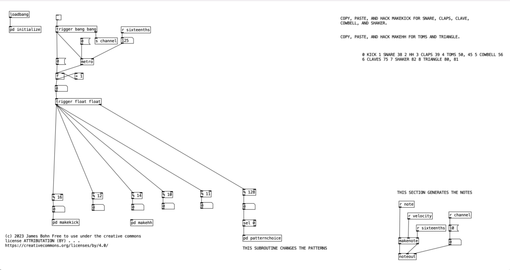
Attached to this blog post is a program shell that we will use to understand a basic process where patterns are defined and initialized, a time structure, a structure for evaluating whether a note should happen, an algorithm for firing off a note, and a structure for changing musical patterns. The way this program shell is designed, it currently only generates kick drum parts in common time. However, once we learn how this algorithm works, we can hack it to create far more complicated beats.
Defining a Pattern

Generating rhythmic content using an algorithm is a very useful exercise, as we do not have to worry about pitch material. On the most basic level, we could think of a measure of as being a list of sixteenth notes (or whatever the fastest pulse of the desired rhythm is), and we can express the rhythm by using zeros where notes do not happen, and ones where notes are played. Thus, if we want to define a four on the floor kick drum part in common time, we could express it as . . .

1 0 0 0 1 0 0 0 1 0 0 0 1 0 0 0

When we define tables in Pure Data, the first number indicates where in the table we’re putting the values. Typically, we would want to start at the beginning of the table, which would be position 0. Thus, from now on in, I will start every rhythm description with a 0, resulting in . . .

0 1 0 0 0 1 0 0 0 1 0 0 0 1 0 0 0

This is pretty basic. If we wanted to go a bit more advanced, we could imagine two different options, a normal kick drum, which we’ll represent with the number 1, and an accented kick drum, which we’ll represent with the number 2. If we want to accent beat one of the measure, we now get the table description . . .

0 2 0 0 0 1 0 0 0 1 0 0 0 1 0 0 0

Notice, it would be pretty easy at this point to use the number zero for when notes do not occur, but use the MIDI velocity number(1-127) to indicate when a note should occur. Doing this, you can get very finely tuned dynamic drum parts. However, such subtlety is not for me, I’m more of a boom / bap / boom-boom / bap guy myself, so I will be sticking with accented and unaccented notes. Let’s look at this table definition as it occurs in the program shell. To get there, double click on the object labeled pd initialize, which is below loadbang . . .
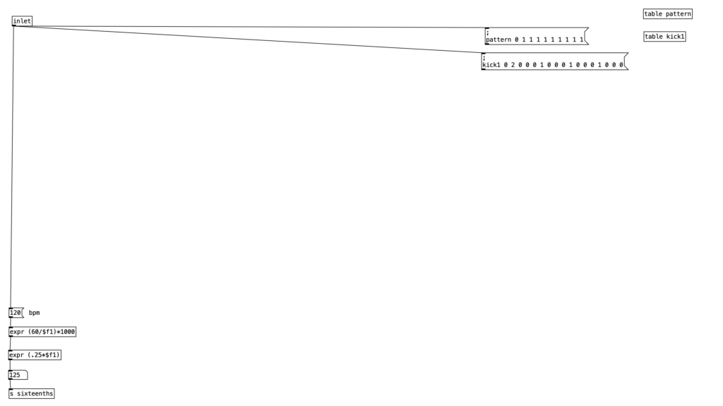
For those who are relatively new to Pure Data, loadbang designates algorithms that execute when you open the program. Likewise, any object in Pure Data that starts with the letters pd are subroutines. Double clicking them allows you to view and edit the algorithm contained inside the subroutine. Subroutines are a great way to declutter your screen, and to create algorithms that you may want to copy and paste into other programs you create. Note that the subroutine pd initialize also sets the tempo, translates that into milliseconds, and then into sixteenth notes (still expressed in milliseconds). Finally, we also see that pd initialize contains a definition for a table called phrase, but we’ll get to that later.

Changing Patterns

Before we get to how to use this kick drum pattern, I want to introduce one more level of complexity. In the long term it would be useful to define several different kick drum patterns so we can change patterns every eight measures or so to have a dynamic drum part. As we start to add more layers to the drum part (snare, high hat, toms, etc.) it would also be nice if some of those layers occasionally did not play at all, so the combination of layers also change as we move from phrase to phrase.

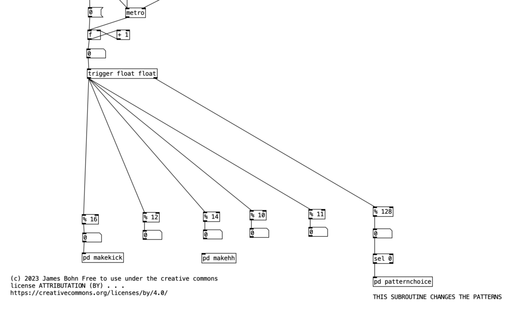
For the purposes of this algorithm, I’m going to allow for each layer of the drum part to select between three patterns (1, 2, & 3). Furthermore, I’ll also include a fourth possibility of 0, which would correspond to no pattern playing. In order to see how this is implemented in our algorithm, let’s look at the counter mechanism beneath the main metronome object. Beneath this metronome we see a trigger object, and beneath that, we see an object that states % 128. This is modular mathematics, which limits the value to a number between 0 and 127 (inclusive). We then feed the outcome of this to an object that states sel 0. When this object receives a 0 in its leftmost inlet, it will send a bang to its leftmost outlet. We then send this bang to trigger the subroutine pd patternchoice. Musically, what this means, is that the subroutine pd patternchoice executes at the beginning of every eight measure phrase. Since we are thinking in terms of sixteenth notes (8 x 16 = 128), a 0 would indicate the beginning of a phrase.
If we look inside pd patternchoice, we see two structures that are currently not connected to the inlet. In time we will copy and paste these structures, changing some of the numeric values, and connect them to the inlet. We will make these changes as we add more layers and patterns to our drum beat. However, for the time being since we only have one kick drum pattern, neither structure is connected to the inlet.
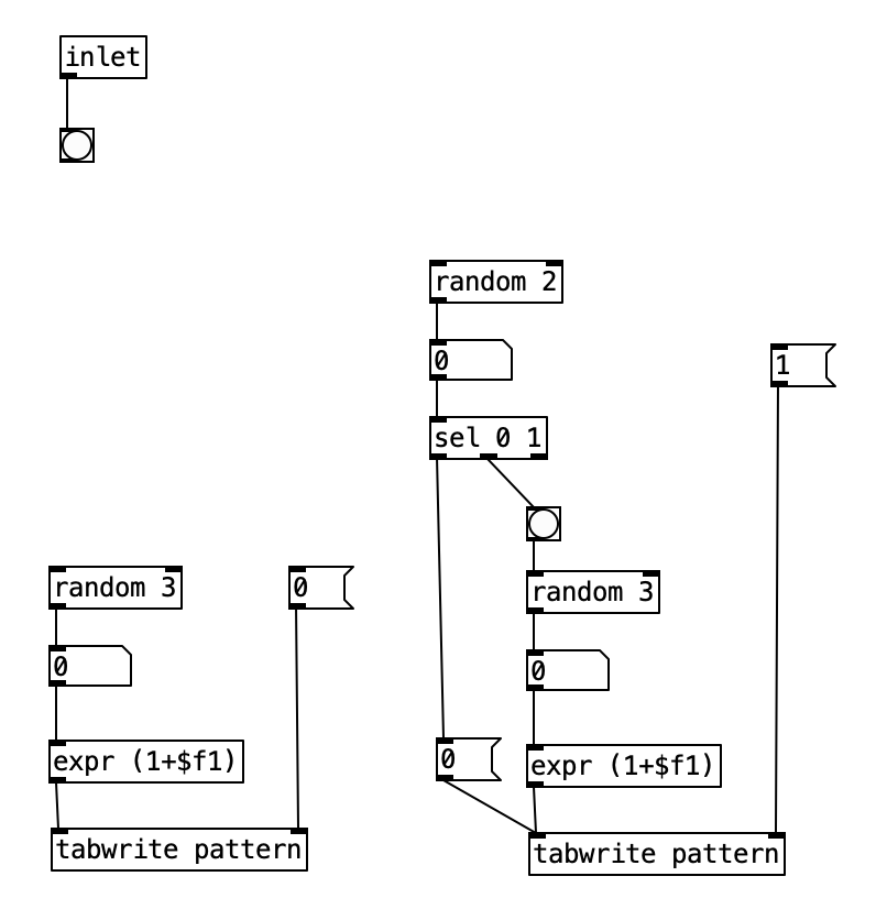
We will treat the algorithm on the left as being connected to the kick drum, while the algorithm on the right will eventually be used for the snare drum. Notice there is a difference between the two structures. The one on the left is simpler, and if we follow what it does, we figure out that that algorithm will write a 1, 2, or 3, but not a 0 to the table pattern in position 0. The structure on the right however, will write a 0 to the table patttern at position 1 half of the time. To put this into musical terms, the difference between the two means that kick drum will always be playing a pattern, while the snare drum will only play a pattern 50% of the time.

Firing Off a Note

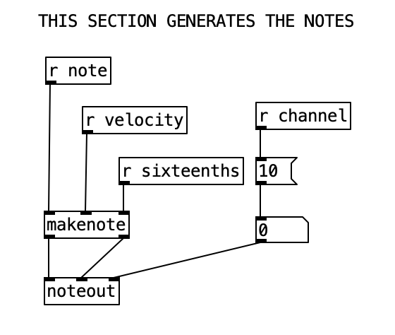
Now lets see how pattern and kick1 are used to either fire off notes or not. We see at the bottom of the screen a makenote object connected to a noteout object that performs the final task of sending a midi note out. However pd makekick is the subroutine that determines whether or not a kick drum should occur at a given point. Above pd makekick we see the object % 16 which comes from the counter. This object mods the current counter to a number between 0 and 15 inclusive. These values correspond to the number of sixteenth notes in a measure of common time. Thus, when we return to the number 0 after the number 15 occurs it corresponds to returning to the beginning of the measure.

When we look at the structure pd makekick a lot of the heavy lifting of the subroutine is handled by the object spigot. Spigot receives numeric values through its leftmost inlet. However, it only passes those values through to its outlet if the numeric value being fed to its right most inlet is not zero. Thus, we can think of spigot as a valve that shuts off the flow of numbers when the rightmost inlet is zero. We can use this to selectively shut down the rest of the algorithm, which will effectively stop it from making notes.
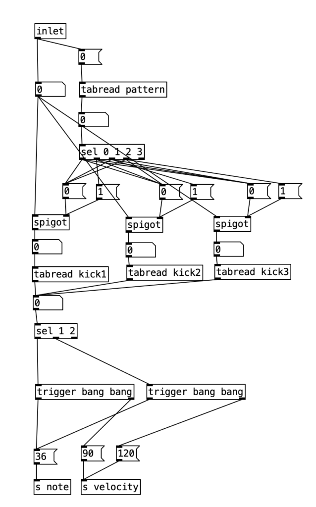
The first step is to determine whether a pattern should be playing or not. Likewise, at the same time we can determine which patterns should be playing if one occurs. To do this, we’ll read the value of pattern at array position 0 (which we’ll use to store the current kick drum pattern). We can then route the output of that to a number of different outcomes using a sel statement. Each outcome of the sel statement sends either a 0 or a 1 to the rightmost inlet of three spigots. These spigots correspond to the three possible kick drum patterns. Thus, when the pattern is 0, a 0 is sent to all three spigots, effectively shutting off the rest of the subroutine. When the pattern is 1, we send a 1 to the spigot for pattern one (turning it on), and a zero to the other two, making sure any previously used pattern is turned off, and so fourth.

Once we pass through one of the spigots, we encounter the part of the subroutine that determines whether a note should be fired at any given time. Underneath each spigot is a tabread object that reads the current position of a given pattern (kick1, kick2, or kick3, respectively). This will return the result of a 0, 1, or 2, corresponding to no note, normal note, and accented note. Since we don’t have to do anything when no note is played, we can simply ignore that result. All we have to do is correctly route the results for 1 and 2. Since all three patterns will be outputing 0, 1, and 2, we will treat those three results the same, we can route the output of each tabread statement to the same number box, and then route the results using sel 1 2. Both results will sending the number 36 to s note (36 is the MIDI note number corresponding to a kick drum), and will send a velocity of either 90 or 120 to s velocity.

Understanding Execution Order

In order to understand the mechanics of this, we have to understand a little about execution order for Pure Data. When an outlet branches off in several directions, Pure Data first executes the connection that was created first, regardless of where it is placed on the screen (in Max, it executes from right to left). When an algorithm branches off in this way, it travels all the way down until it hits the end, and then Pure Data goes back and executes the other branch of the algorithm. When an object has multiple outlets, it typically executes the rightmost outlet first (following it all the way down the algorithm) before it most to the next outlet.

Alternately, when an object has several inlets, the object typically does not spring into action until the leftmost inlet is triggered. We can think of new values that are connected to inlets that are note the leftmost inlet as queueing until the leftmost inlet is triggered. This order of execution in Pure Data allows non-crossed connections to fire in the correct order. To illustrate, imagine an object with two outlets and an object below with two inlets (similar to the makenote / noteout algorithm below). Furthermore, let’s imagine that the right outlet is connected to the right inlet of the object below, and the left outlet is connected to the left inlet of the object below. First, the value from the right outlet will queue at the right inlet of the object below, then the left outlet will send its value to the left inlet, triggering the object below.
However, whenever we start to make complicated algorithms, it can be confusing to see in what order the algorithm will flow. When we want to force a specific order to achieve a specific outcome, or simply to make order clear, we can use a trigger object. A trigger takes a single inlet, and uses it to trigger several outlets (including the option of passing the inlet to one or more outlets) in a specific order. That order is (you guessed it, right to left). We will use this to control the order of sending the velocity and sending the note number.
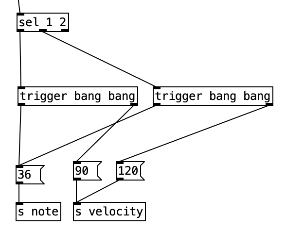
The makenote object has three inlets that correspond to midi note number, velocity, and duration expressed in milliseconds. Since midi note number is the leftmost inlet, we have to send that value last. This means we have to send the velocity before we send the note number. Here we do not have to worry about duration, since duration is often irrelevant when triggering drum samples. Thus, we can set a duration of a sixteenth note during the initialization process.

Hacking the Shell

With the knowledge we have gained thus far, we are now equipped to start hacking the program shell. A good place to start would be to double click [pd initialize], copy both the object [table kick1] and the corresponding message that populates that table. You can then paste these objects, move them so they don’t overlap, change both to say kick2 instead of kick1, and change the numbers in the in the kick2 message to be a different pattern. Again, your pattern should only use the numbers 0, 1, and 2. Likewise, the table should be 17 numbers long with the first number being 0, in order to denote that we’ll load the array starting at the beginning. You can then connect the kick2 message to the [inlet] object.

Now do the same process again creating a table and message for kick3, making sure to connect the kick3 message to inlet. Now, we can finally make use of the subroutine [pd patternchoice] in the main algorithm. Double click on [pd patternchoice], and connect the outlet of the bang to both the [random 3] object and the message that contains the number 0. Now, when we run the the algorithm, we should hear the kick drum pattern randomly change once every eight measures.

Now we can get into the good stuff. Let’s add a snare drum part. First, we should decide what meter we want to use for the snare drum. For the purposes of this demonstration, let’s put the snare drum in three. We’ll start by copying the object [pd makekick] and pasting it. More the copied object under the [% 12] object, and connect the outlet of [% 12] to the inlet of the copied object. Let’s also rename the copied object to [pd makesnare].

We have to change some details of [pd makesnare] to get it to make a snare part. Double click the object and change the message box near the top from 0 to 1. Change the array names in the three [tabread] objects to be snare1, snare2, and snare3. Finally, right above the object [s note], change the number in the message box from 36 to 38 (the MIDI note number for snare drum).

Now, double click the object [initialize], and copy the three kick drum tables, as well as the three messages that define those tables. Paste those items, and move them so they don’t overlap with other items. change the array names to snare1, snare2, and snare3 in both the table objects and the messages that define the arrays. Now, let’s change the patterns. Since these are patterns that are in three, they will feature 12 sixteenth notes. Thus, each message will have to include 13 numbers, the first being the number 0 to indicate that the pattern is loaded at the beginning of the array. Again, use 0 to indicate no note, 1 to indicate a note, and 2 to represent an accented note. Make sure you connect each of the three messages to the inlet.

Now we need to allow the snare patterns to change, so let’s double click the subroutine [pd patternchoice]. In this subroutine we need to connect the outlet of the bang to both the [random 2] object and the message that contains the number 1. The [random 2] here yields a 50% chance that the snare appear in a given phrase. The [random 3] below that will select one of the three snare patterns when it is determined that the snare should appear in a phrase.

Experiment 10: Five EYESY Algorithms

I kind of hit a wall of the Organelle. I feel like in order to advance my skills I have a bit of a hurdle between where my programming skills are at, and where they would need to be to do something more advanced that the recent experiments I have completed. Accordingly for this month I decided to shift my focus to the EYESY. Last month I made significant progress in understanding Python programming for the EYESY, and that allowed me to come up with five ideas for algorithms in short order. The music for all five mini-experiments comes from PureData algorithms I will be using for my next major album. All five of these algorithms are somewhat derived from my work on my last album.

The two realizations that allowed me to make significant progress on EYESY programming is that Python is super picky about spaces, tabs, and indentations, and that while the EYESY usually gives little to no feedback when a program has an error in it, you can use an online Python compiler to help figure out where your error is (I had mentioned the latter in last month’s experiment). Individuals who have a decent amount of programming experience may scoff at the simplicity of the programs that follow, but for me it is a decent starting place, and it is also satisfying to me to see how such simple algorithms can generate such gratifying results.

Random Lines is a patch I wrote that draws 96 lines. In order to do this in an automated fashion, I have to use a loop, in this case I use for i in range(96):. The five lines that follow are all executed in this loop. Before the loop commences, we choose the color using knob 4 and the background color using knob 5. I use knob 3 to set the line width, but I scale it by multiplying the knob’s value, which will be between 0 and 1, by 10, and adding 1, as line widths cannot have a value of 0. I also have to cast the value as an integer. I set an x offset value using knob 1. Multiplying by 640 and then subtracting 320 will yield a result between -320 and 320. Likewise, a y offset value is set using knob 2, and the scaling results in a value between -180 and 180.

import os
import pygame
import time
import random
import math

def setup(screen, etc):
    pass

def draw(screen, etc):
	color = etc.color_picker(etc.knob4)
	linewidth = int (1+ (etc.knob3)*10)
 	etc.color_picker_bg(etc.knob5)
	xoffset=(640*etc.knob1)-320
	yoffset=(360*etc.knob2)-180
   	for i in range(96):
		x1 = int (640 + (xoffset+(etc.audio_in[i])/50))
		y1 = int (360 + (yoffset+(etc.audio_in[(i+1)])/90))
		x2 = int (640 + (xoffset+(etc.audio_in[(i+2)])/50))
		y2 = int (360 + (yoffset+(etc.audio_in[(i+3)])/90))
		pygame.draw.line(screen, color, (x1,y1), (x2, y2), linewidth)

Within the loop, I set two coordinates. The EYESY keeps track of the last hundred samples using etc.audio_in[]. Since these values use sixteen bit sound, and sound has peaks (represented by positive numbers) and valleys (represented by negative numbers), these values range between -32,768 and 32,787. I scale these values by dividing by 50 for x coordinates. This will scale the values to somewhere between -655 and 655. For y coordinates I divide by 90, which yields values between -364 and 364.

In both cases, I add these values to the corresponding offset value, and add the value that would normally, without the offsets, place the point in the middle of the screen, namely 640 (X) and 360 (Y). A negative value for the xoffset or the scaled etc.audio_in value would move that point to the left, while a positive value would move it to the right. Likewise, a negative value for the yoffset or the scale etc.audio_in value would move the point up, while a positive value would move it down.

Since subsequent index numbers are used for each coordinate (that is i, i+1, i+2, and i+3), this results in a bunch of interconnected lines. For instance when i=0, the end point of the drawn line (X2, Y2) would become the starting point when i=2. Thus, the lines are not fully random, as they are all interconnected, yielding a tangled mass of lines.

Random Concentric Circles uses a similar methodology. Again, knob five is use to control the background color, while knobs 1 and 2 are again scaled to provide an X and Y offset. The line width is shifted to knob 4. For this algorithm the loop happens 94 times. The X and Y value for the center of the circles is determined the same way as was done in Random Lines. However, we now need a radius and we need a color for each circle.

import os
import pygame
import time
import random
import math

def setup(screen, etc):
    pass

def draw(screen, etc):
	linewidth = int (1+(etc.knob4)*9)
 	etc.color_picker_bg(etc.knob5)
	xoffset=(640*etc.knob1)-320
	yoffset=(360*etc.knob2)-180
	for i in range(94):
		x = int (640 + xoffset+(etc.audio_in[i])/50)
		y = int (360 + yoffset+(etc.audio_in[(i+1)])/90)
		radius = int (11+(abs (etc.knob3 * (etc.audio_in[(i+2)])/90)))
		r = int (abs (100 * (etc.audio_in[(i+3)]/33000)))
		g = int (abs (100 * (etc.audio_in[(i+4)]/33000)))
		b = int (abs (100 * (etc.audio_in[(i+5)]/33000)))
		thecolor=pygame.Color(r,g,b)
		pygame.draw.circle(screen, thecolor, (x,y), radius, linewidth)

We have knob 3 available to help control the radius of the circle. Here I multiply knob 3 by a scaled version of etc.audio_in[(i+2)]. I scale it by dividing by 90 so that the largest possible circle will mostly fit on the screen if it is centered in the screen. Notice that when we multiply knob 3 by etc.audio_in, there’s a 50% chance that the result will be a negative number. Negative values for radii don’t make any sense, so I take the absolute value of this outcome using abs. I also add this value to 11, as a radius of 0 makes no sense, and a radius of less than 10, as having a line width that is larger than the radius will cause an error.

For this algorithm I take a set forward by giving each circle its own color. In order to do this I have to set the value for red, green, and blue separately, and then combine them together using pygame.Color(). For each of the three values (red, green, and blue) I divide a value of etc. audio_in by 33000, which will yield a value between 0 and 1 (more or less), and then multiply this by 100. I could have done the same thing by simply dividing etc.audio_in by 330, however, at the time this process made the most sense to me. Again, this process could result in a negative number and / or a fractional value, so I cast the result as an integer after getting its absolute value.

Colored Rectangles has a different structure than the previous two examples. Rather than have all the objects cluster around a center point I wanted to create an algorithm that spaces all of the objects out evenly throughout the screen in a grid like pattern. I do this using an eight by eight grid of 64 rectangles. I accomplish the spacing using modulus mathematics as well as integer division. The X value is obtained by multiplying 160 times i%8. In a similar vein, the Y values is set to 90 times i//8. Integer division in Python is accomplished through the use of two slashes. Using this operator will return the integer value of a division problem, omitting the fractional portion. Both the X and the Y values have an additional offset value. The X is offset by (i//8)*(80*etc.knob1), so this offset increases as knob 1 is turned up, with a maximum offset of 80 pixels per row. The value i//8 essentially multiplies that offset by the row number. That is the rows shift further towards the right.

import os
import pygame
import time
import random
import math

def setup(screen, etc):
    pass

def draw(screen, etc):
 	etc.color_picker_bg(etc.knob5)
   	for i in range(64):
		x=(i%8)*160+(i//8)*(80*etc.knob1)
		y=(i//8)*90+(i%8)*(45*etc.knob2)
		thewidth=int (abs (160 * (etc.knob3) * (etc.audio_in[(i)]/33000)))
		theheight=int (abs (90 * (etc.knob4) * (etc.audio_in[(i+1)]/33000)))
		therectangle=pygame.Rect(x,y,thewidth,theheight)
		r = int (abs (100 * (etc.audio_in[(i+2)]/33000)))
		g = int (abs (100 * (etc.audio_in[(i+3)]/33000)))
		b = int (abs (100 * (etc.audio_in[(i+4)]/33000)))
		thecolor=pygame.Color(r,g,b)
		pygame.draw.rect(screen, thecolor, therectangle, 0)

Likewise, the Y offset is determined by (i%8)*(45*etc.knob2). As the value of knob 2 increases, the offset moves towards a maximum value of 45. However, as the columns shift to the right, those offsets compound due to the fact that they are multiplied by (i%8).

A rectangle can be defined in pygame by passing an X value, a Y value, width, and height to pygame.Rect. Thus, the next step is to set the width and height of the rectangle. In both cases, I set the maximum value to 160 (for width) and 90 (for height). However, I scaled them both by multiplying by a knob value (knob 3 for width and knob 4 for height). These values are also scaled by an audio value divided by 33,000. Since negative values are possible from audio values, and negative widths and heights don’t make much sense, I took the absolute value of each. If I were to rewrite this algorithm (perhaps I will), I would set a minimum value for width and height such that widths and heights of 0 were not possible.

I set the color of each rectangle using the same method as I did in Random Concentric Circles. In order to draw the rectangle you pass the screen, the color, the rectangle (as defined by pygame.Rect), as well as the line width to pygame.draw.rect. Using a line width of 0 means that the rectangle will be filled in with color.

Random Rectangles is a combination of Colored Rectangles and Random Lines. Rather than use pygame’s Rect object to draw rectangles on the screen, I use individual lines to draw the rectangles (technically speaking they are quadrilaterals). Knob 4 is used here to set the foreground color, knob 5 is used here to set the background color, knob 3 is used to set the linewidth.

import os
import pygame
import time
import random
import math

def setup(screen, etc):
    pass

def draw(screen, etc):
	color = etc.color_picker(etc.knob4)
 	etc.color_picker_bg(etc.knob5)
	linewidth = int (1+ (etc.knob3)*10)
   	for i in range(64):
		x=(i%8)*160+(i//8)*(80*etc.knob1)+(40*(etc.audio_in[(i)]/33000))
		y=(i//8)*90+(i%8)*(45*etc.knob2)+(20*(etc.audio_in[(i+1)]/33000))
		x1=x+160+(40*(etc.audio_in[(i+2)]/33000))
		y1=y+(20*(etc.audio_in[(i+3)]/33000))
		x2=x1+(40*(etc.audio_in[(i+4)]/33000))
		y2=y1+90+(20*(etc.audio_in[(i+5)]/33000))
		x3=x+(40*(etc.audio_in[(i+6)]/33000))
		y3=y+90+(20*(etc.audio_in[(i+7)]/33000))
		pygame.draw.line(screen, color, (x,y), (x1, y1), linewidth)
		pygame.draw.line(screen, color, (x1,y1), (x2, y2), linewidth)
		pygame.draw.line(screen, color, (x2,y2), (x3, y3), linewidth)
		pygame.draw.line(screen, color, (x3,y3), (x, y), linewidth)

Within the loop, I use a similar method of setting the initial X and Y coordinates. That being said, I separate out the use of knobs and the use of audio input. In the case of the X coordinated, I use (i//8)*(80*etc.knob1) to control the amount of x offset for each row, with a maximum offset of 80. The audio input then offsets this value further using (40*etc.audio_in[(i+2)]/33000). This moves the x value by a value of plus or minus 40 (remember that audio values can be negative. Likewise, knob 2 offsets the Y value for every row by a maximum of 45, and the audio input further offsets this value by plus or minus 20.

Since it takes four points to define a quadrilateral, we need three more points, which we will call (x1, y1), (x2, y2), and (x3, y3). These are all interrelated. The value of X is used to define X1 and X3, while X2 is based off of X1. Likewise, the value of Y helps define Y1 and Y3, with Y2 being based off of Y1. In the case X1 and X2 (which is based on X1) we add 160 to X, giving a default width, but these values are again scaled by etc.audio_in. Similarly, we add 90 to Y1 and Y3 to determine a default height of the quadrilaterals, but again, all points are further offset by etc.audio_in, resulting in quadrilaterals, rather than rectangles with parallel sides. If I were to revise this algorithm I would likely make each quadrilateral a different color.

Frankly, I was not as pleased with the results of Colored Rectangles and Random Rectangles, so I decided to go back create an algorithm that was an amalgam of Random Lines and Random Concentric Circles, namely Random Radii. This program creates 95 lines, all of which have the same starting point, but different end points. Knob 5 sets the background color, while knob 4 sets the line width.

import os
import pygame
import time
import random
import math

def setup(screen, etc):
    pass

def draw(screen, etc):
	linewidth = int (1+ (etc.knob4)*10)
 	etc.color_picker_bg(etc.knob5)
	xoffset=(640*etc.knob1)-320
	yoffset=(360*etc.knob2)-180
	X=int (640+xoffset)
	Y=int (360+yoffset)
   	for i in range(95):
		r = int (abs (100 * (etc.audio_in[(i+2)]/33000)))
		g = int (abs (100 * (etc.audio_in[(i+3)]/33000)))
		b = int (abs (100 * (etc.audio_in[(i+4)]/33000)))
		thecolor=pygame.Color(r,g,b)
		x2 = int (640 + (xoffset+etc.knob3*(etc.audio_in[(i)])/50))
		y2 = int (360 + (yoffset+etc.knob3*(etc.audio_in[(i+1)])/90))
		pygame.draw.line(screen, thecolor, (X,Y), (x2, y2), linewidth)

Knob 1 & 2 are used for X and Y offsets (respectively) of the center point. Using (640*etc.knob1)-320 means that the X value will move plus or minus 320. Similarly, (360*etc.knob2)-180 permits the Y value to move up or down by 180. As is the case with Random Concentric Circles, the color of each line is defined by etc.audio_in. Knob 3 is used to scale the end point of each line. In the case of both the X and Y values, we start from the center of the screen (640, 360) add the offset defined by knobs 1 or 2, and then use knob 3 to scale a value derived from etc.audio_in. Since audio values can be positive or negative, these radii shoot outward from the offset center point in all directions.

As suggested earlier, I am very gratified with these results. Despite the simplicity of the Python code, the results are mostly dynamic and compelling (although I am somewhat less than thrilled with Colored Rectangles and Random Rectangles). The user community for the EYESY is much smaller than that of the Organelle. The EYESY user’s forum has only 13% the activity of that of the Organelle. I seem to have inherited being the administrator of the ETC / EYESY Video Synthesizer from Critter&Guitari group on Facebook. Likewise, I am the author of the seven most recent patches for the EYESY on patchstorage. Thus, this month’s experiment sees me shooting to the top to become the EYESY’s most active developer. The start of the semester has been very busy for me. I am somewhat doubting that I will be coming up with an Organelle patch next month, but I equally suspect that I will continue to develop more algorithms of the EYESY.

Experiment 8: Bass Harmonica

For this month’s experiment I created a sample player that triggers bass harmonica samples. I based the patch off of Lo-Fi Sitar by a user called woiperdinger. This patch was, in turn, based off of Lo-Fi Piano by Henr!k. According to this user, this was based upon a patch called Piano48 by Critter and Guitari.

The number 48 in the title refers to the number of keys / samples in the patch. Accordingly, my patch has the potential for 48 different notes, although only 24 notes are actually implemented. This is due to the fact that the bass harmonica I used to create the sample set only features 24 pitches. I recorded the samples using a pencil condenser microphone. I pitch corrected each note (my bass harmonica is fairly out of tune at this point), and I EQed each note to balance the volumes a bit. Initially I had problems as I had recorded the samples at a higher sample rate (48kHz) than the Organelle operates at (44.1kHz). This resulted in the pitch being higher than planned, but it was easily fixed by adjusting the sample rate on each sample. I had planned on recording the remaining notes using my Hohner Chromonica 64, but I ran out of steam. Perhaps I will expand the sample set in a future release.

The way this patch works is that every single note has its own sample. Furthermore, each note is treated as its own voice, such that my 24 note bass harmonica patch allows all 24 notes to be played simultaneously. The advantage of having each note have its own sample is that each note will sound different, allowing the instrument to sound more naturalistic. For instance the low D# in my sample set is really buzzy sounding, because that note buzzes on my instrument. Occasionally hitting a note with a different tone color makes it sound more realistic. Furthermore, none of the samples have to be rescaled to create other pitches. Rescaling a sample either stretches the time out (for a lower pitch) or squashes the time (for a higher pitch), again creating a lack of realism.

The image above looks like 48 individual subroutines, but it is actually 48 instantiations of a single abstraction. The abstraction is called sampler-voice, and each instance of this abstraction is passed the file name of the sample along with the key number that triggers the sample. The key numbers are MIDI key numbers, where 60 is middle C, and each number up or down is one chromatic note away (so 61 would be C#).

Inside sampler-voice we see basically two algorithms, one that executes when the abstraction loads (using loadbang), and one that runs while the algorithm is operating. If we look at the loadbang portion of the abstraction, we see that it uses the object soundfiler to load the given sample into an array. This sample is then displayed in the canvas to the left. Soundfiler sends the number of samples to its left outlet. This number is then divided by 44.1 to yield the time in milliseconds.

As previously stated, the balance of the algorithm operates while the program is running. The top part of the algorithm, r notes, r notes_seq, r zero_notes, listens for notes. The object stripnote is being used to isolated the MIDI note number of the given event. This is then passed through a mod (%) 48 object as the instrument itself only has 48 notes. I could have changed this value to 24 if I wanted every sample to recur once every two octaves. The object sel $2 is then use to filter out all notes except the one that should trigger the given sample ($2 means the second value passed to the abstraction). The portion of the algorithm that reads the sample from the array is tabread4~ $1-array.

Knob 1 of the Organelle is used to control the pitch of the instrument (in case you want to transpose the sample). The second knob is used to control both the output level of the reverb as well as the mix between the dry (unprocessed) sound and the wet (reverberated) sound. In Lo-Fi Sitar, these two parameters each had their own knob. I combined them to allow for one additional control. Knob 3 is a decay control that can be used if you don’t want the whole sample to play. The final knob is used to control volume, which is useful when using a wind controller, such as the Warbl, as that can be used to allow the breath control to control the volume of the sample.

The PureData patch that controls the accompaniment is basically the finished version of the patch I’ve been expanding through this grant project. In addition to the previously used meters 4/4, 3/4, and 7/8, I’ve added 5/8. I’d share information about the algorithm itself, but it is just more of the same. Likewise, I haven’t done anything new with the EYESY. I’m hoping next month I’ll have the time to tweak an existing program for EYESY, but I just didn’t have the time to do that this month.

I should have probably kept the algorithm at a slower tempo, as I think the music works better at a slower tempo. The bass harmonica samples sound fairly natural, except for when the Organelle seems to accidentally trigger multiple samples at once. I have a theory that the Warbl uses a MIDI On message with a velocity of 0 to stop notes, which is an acceptable use of a MIDI On message, but that PureData uses it to trigger a note. If this is the case, I should be able to fix it in the next release of the patch.

It certainly sounds like I need to practice my EVI fingering more, but I found the limited pitch range (two octaves) of the sample player made the fingering easier to keep track of. Since you cannot use your embouchure with an EVI, you use range fingerings in order to change range. With the Warbl, your right hand (lower hand) is doing traditional valve fingerings, while your left hand (upper hand) is doing fingerings based upon traditional valve fingerings to control what range you are playing on. Keeping track of how the left hand affects the notes being triggered by the right hand has been my stumbling block in terms of learning EVI fingering. However, a two octave range means you really only need to keep track of four ranges. I found the breath control of the bass harmonica samples to be adequate. I think I’d really have to spend some time calibrating the Warbl and the Organelle to come up with settings that will optimize the use of breath control. Next month I hope to create a more fanciful sample based instrument, and maybe move forward on programming for the EYESY.

Experiment 2: Analog Style


May has been a busy month for me. Thus, my second experiment in my project funded by Digital Innovation Lab at Stonehill College investigates the use of the preset patch Analog Style (designed by Critter and Guitari). To be specific, I am using a WARBL wind controller with EVI fingering to control the patch. I am using the breath control on the WARBL to control the cutoff frequency of Analog Style (using MIDI controller 24).

Due to the busyness of the end of the semester, this experiment features no original programming on the organelle. However, I did create a program in Pure Data to create accompaniment and drive the EYESY. To accompany the experiment, I used the H.E.A.P, the Housatonic Electronic Algorithmic Philharmonic. This a fun, frivolous name I’ve given to a small, battery powered synthesizer / sampler setup I’ve assembled for live performance. It consists of three synthesizers / samplers: a Volca Sample 2 (which provides 10 channels of late 1980s style lo fidelity digital sampling), a Volca Keys (which can be used as an analog monophonic or 3 note polyphonic synthesizer), and a Volca FM 2 (which is a clone of the 1980s classic, the Yamaha DX7, the best selling synthesizer of all time). I’ve also begun to think of the EYESY, as we’ll see later, as part of the H.E.A.P.

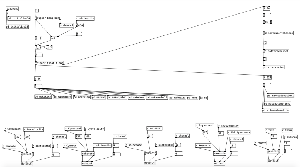
I won’t go into great detail about the program that generates the accompaniment for Experiment 2, as I have other blog posts that go into detail about various algorithms included in the program. Ultimately, the program is intended to generate relatively generic, but fairly usable R&B esque slow jams. The music is in common time using sixteenth notes. The portion of the program including and beneath % 16 (mod 16) ensures that the resulting music will have 16 pulses per measure. Likewise, the instrumentation and musical patterns change every four measures. This is enabled by the part of the program including and beneath % 64 (four measures of sixteenth notes adds up to 64).

The Volca Sample is being used to provide the drum beat, and some string pizzicato (see pd makepizz). The Volca Keys provides some synthesized bass patterns that run two measure loops. The Volca FM provides four chord, four note chord progressions that repeat every two measures. To create these chord progressions I used some music programming techniques that I’ve covered in a previous blog entry, though in this experiment I am use the brass friendly key of G minor.

One of the newer programming tricks I used in this program is an algorithm designed to drive the EYESY. While the EYESY generates hypnotic, interactive video animations, left to its own devices it can get a bit repetitive fairly quickly. In order to generate anything that seems even remotely dynamic some one needs to perform the EYESY by rotating its five knobs. This is an impossibility for any performing musician, save for a vocalist. Thankfully, we can do the equivalent of turning the knobs on the EYESY through MIDI using controllers 21 through 25.

The algorithm I’ve created to drive the EYESY is designed to make slow, evolving changes. To control these changes I’ve created a table called videostatus. It consists of five positions that contain a one or a zero to denote whether changes should be make or not made to a given knob during the current four measure phrase.

The subroutine pd videochoice is triggered at the beginning of every four measure phrase. It generates five different random numbers that are either a zero or a one. These results are then stored in the table videostatus.

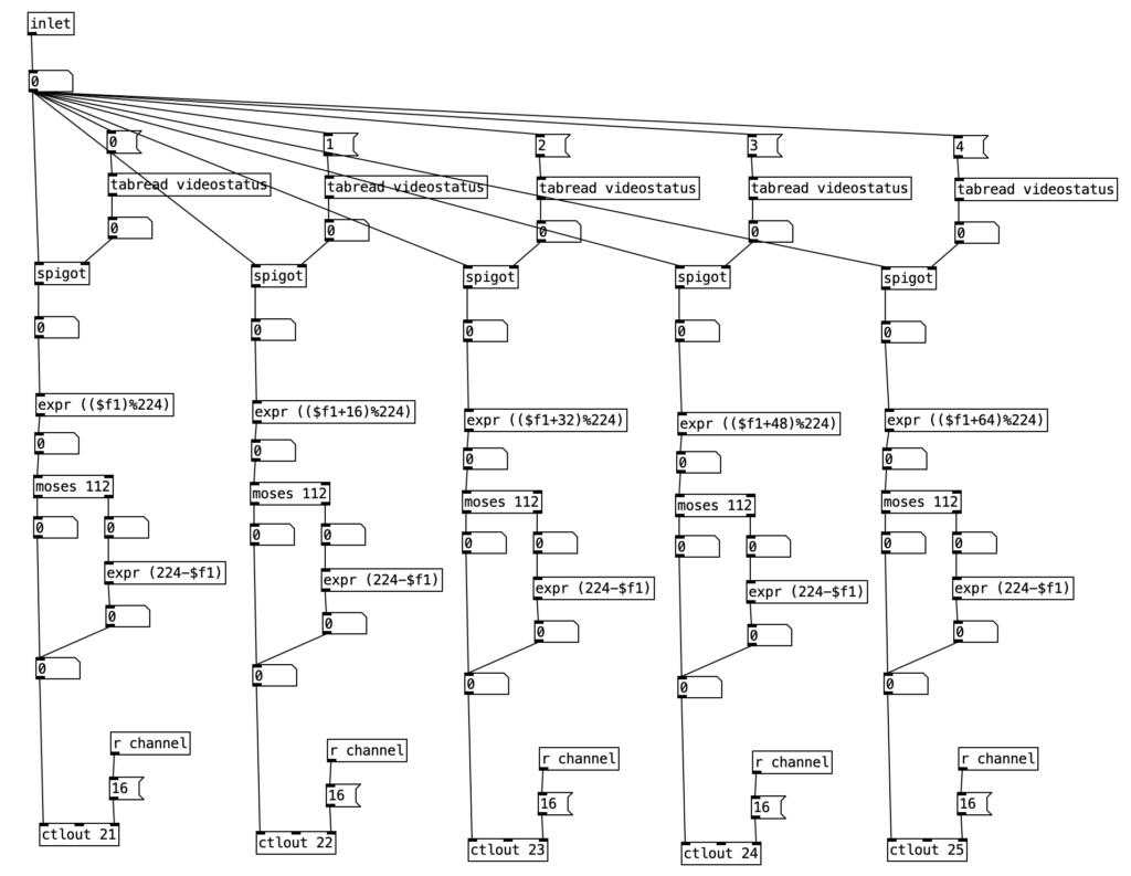
The subroutine pd videoautomation updates the knob positions on the EYESY once every sixteenth note. It is passed the current sixteenth note number modded by the number 224, which corresponds to 14 measures of sixteenth notes. The subroutine contains five nearly identical columns, each of which corresponds to each of the five knobs on the EYESY. First the algorithm checks the current states of each of the five positions of videostatus table. When that value is one, that allows the current sixteenth note number to pass through the spigot. This value is passed through an expr statement that displaces the sixteenth note number. The column corresponding to knob one is not displaced, but each subsequent column is displaced by one measure (16 sixteenths), which is then modded to stay between 0 and 224. The statement moses 112 is used to determine whether we should be counting up to 112, or counting down to 0. This is accomplished by having numbers that are greater than 112 to pass through expr (224-$f1), which causes the result to get small as the input value is increased. The result of this is then passed to one of the five controller values (21-25) on MIDI channel 16 (the channel I’ve set my EYESY to).

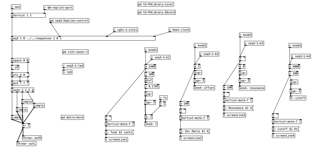
Since I went over the mother patch in the previous experiment, I’ll start with going over main.pd for the Analog Style patch. We can see that knob one controls the tuning of the patch, while knob two creates an offset frequency for a second oscillator. The third knob sets the resonance of the low pass filter, while the fourth knob (the one I am controlling using the WARBL) sets the cutoff frequency of filter. To learn more about what low pass filters are, check out my blog entry on Low Pass Filters in LogicPro. However, to summarize briefly in relationship to the WARBL, when the amount of breath coming through is low, that in turn sets the cutoff frequency to be low as well, resulting in less sound (and only low frequency sound) to come out of the Organelle.

We can also see that this patch allows for sequencing when the aux button is down. However we will not go through how sequencing works today. We will however go into simple, which is the subroutine that creates the sound. We can see two oscillators, blsaw, in this subroutine that generate sawtooth waves. For more information on subtractive synthesis waveforms (including sawtooth waves), check out my blog entry on Subtractive Synthesis Waveforms in Logic Pro. One of those two blsaw oscillators is modified by the offset of knob two. The mixture of these two oscillators is passed to a low pass filter, moog~. This object also receives a center frequency to its center inlet, and a resonance value to its right most inlet. The outlet of this object is then attenuated slightly, *~ .75, before being sent to the subroutine’s outlet.

Again, I’ve found that the accompaniment generated by experiment.pd to be generic, but also fairly usable. It should be relatively easy to change the tempo, phrase length, or any number of musical patterns to create music that is stylistically different. Also, I enjoy slow evolving nature of EYESY generated video. I feel that turning on and off changes to various combinations of the five knobs add a degree of subtlety that aid in the dynamic nature of the video.

I am disappointed in my performance on the WARBL. I am still getting used to the EVI fingering on the instrument, so there are some very sour notes from time to time. However, I am very pleased with the range of the WARBL, as well as the subtle breath control the instrument provides. The fingering makes jumping octaves and fifths very easy. In future experiments I hope to get into hacking existing Organelle patches. I also plan to come up with variants of the videoautomation algorithm to create more sudden, less subtle changes to the EYESY’s settings.

Pure Data: Scale Sequencer

Inspired by the book Learning Music Theory With Logic, Max, And Finale by Geoffrey Kidde, I have decided to revise my curriculum in my entry level theory course. However, rather than use Max, I’ve opted to teach Pure Data, due to its low price ($0). Pure Data is just different enough from Max that you can’t really use teaching materials for the two programs interchangeably. Thus, teaching Pure Data is forcing me to learn it, which is something I’ve wanted to do for quite a while. I hope to put up occasional posts that share Pure Data patches that I have developed for my teaching.

The first of these is a patch that plays major scales in three different octaves, at three different speeds.

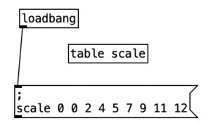
Let’s look at this patch in a little detail. For those who are new to Pure Data, loadbang is used to run part of your patch when that patch is loaded. This loadbang routine sets up a table called scale, and defines the scale. Note that I’m using numbers of half steps to define a major scale (0 2 4 5 7 9 11 12). Notice as well that there is seemingly an extra 0 at the beginning. However, that first 0 indicates where in the table you begin loading material, so if we were to write this as text, we’d say begin at position 0 (the start of the table), and load in 0, 2, 4, 5, 7, 9, 11, and 12. This table data is included in a message object, and starts with a semicolon followed by a return character.  We would change the data in this message to change the mode or type of scale desired. If you want to update the patch after adding or changing information in the message that defines the scale, all you have to do is click on the message object when not in edit mode.

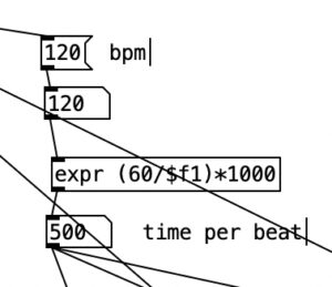
The following segment of the patch translates a tempo, measured in beats per minute to a time per beat measured in milliseconds. The equation expr (60/$f1)*1000 casts the number in the inlet (120) to a float. It divides 60 by that number, resulting in half a second. Multiplying that by 1000 translates that time per beat to milliseconds.

Directly beneath this segment there are three segments that instantiate metronomes at the quarter, eighth, and sixteenth note levels respectively. The quarter note metronome is passed the outlet of the time per beat. For the eighth notes, that same output is halved using expr (.5*$f1). Likewise, the sixteenth note durations result by multiplying by 1/4, using expr (.25*$f). In each case, a duration is also sent (dur1dur2dur3).

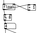
Below the metronomes are counters. The top two objects are very commonly used in Pure Data. The object on the left creates and stores a floating point number (a number with a decimal). To the right, we have an object that increments that number by adding one. This is accomplished by feeding the outlet of the float to the inlet of “+ 1”, and feeding the outlet of “+ 1” into the right inlet sets a new value for the float.

Since a scale has eight notes, any number higher than this is fairly useless for generating a scale. Thus, the outlet of float also feeds to “% 8”. The percentage sign means mod (modulus mathematics). Technically speaking, what is happening here is the number being fed to “% 8” is divided by eight, but the remainder of that division (the number that is left over in whole number division) is then sent to the outlet. This will result in a number between zero and seven.

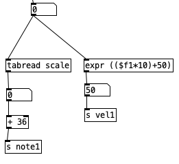
This number is then used to generate both a pitch and a velocity. It is used as an index to select a value out of the the scale table, which is then added to a base pitch to determine the pitch range. The quarter notes use note number 36 as the base pitch. Since middle C (C4) in MIDI (Musical Instrument Digital Interface) is 60, 36 would be two octaves beneath middle C, otherwise known as C2, or Cello C. The eighth notes use middle C (60) as its base, and the sixteenth notes use two octaves above middle C (C6 or 84) as its base pitch. The pitch is then sent via the send command (s for short) using the variables note1, note2, and note3 for the quarters, eighths, and sixteenths respectively.

Key velocity in MIDI is a measurement of how quickly a key is pressed down. Traditionally it is used to indicate how loud a note is. That is a key that is pressed quickly will be louder than a key that is depressed slowly. MIDI is largely a seven bit system, so velocity values run between zero (which also can be used to turn a note off), and 127 (which is the loudest a note can be played). The equation expr (($f1*10)+50) results in having the notes get louder as the pitch of the scale goes up. For instance, when the index is zero, the velocity will be 50, and when the index is seven, the velocity will be 120.

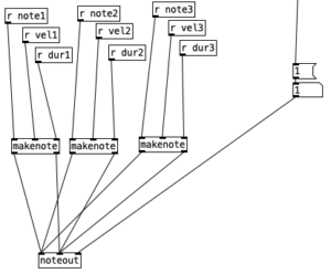
These values, the notes (note1, note2, note3) and the velocities (vel1, vel2, vel3), are then sent to the output stage. The object makenote receives in its inlets (left to right) MIDI note number, velocity (0-127), and duration (in milliseconds). The outlets of makenote then feed the two leftmost inlets of noteout. The rightmost inlet of noteout receives a MIDI channel. The original specifications for MIDI, which was released in 1983, allow for 16 MIDI channels. Here, the notes are being sent on the first channel. Three different instances of makenote are being used here to allow different velocities and durations to be happening simultaneously.

You may check out this patch in action below using a piano sampler from Apple’s LogicPro to realize the sound.