Experiment 11: Constellations

February was a very busy month for me for family reasons, and it’ll likely be that way for a few months. Accordingly, I’m a bit late on my February experiment, and will likely be equally late with my final experiment as well. I have also stuck with programming for the EYESY, as I have kind of been on a roll in terms of coming up with ideas for it.

This month I created twelve programs for the EYESY, each of which displays a different constellation from the zodiac. I’ve named the series Constellations and have uploaded them to patchstorage. Each one works in exactly the same manner, so we’ll only look at the simplest one, Aries. The more complicated programs simply have more points and lines in them with different coordinates and configurations, but are otherwise are identical.

Honestly, one of the most surprising challenges of this experiment way trying to figure out if there’s any consensus for a given constellation. Many of the constellations are fairly standardized, however others are fairly contested in terms of which stars are a part of the constellation. When there were variants to choose from I looked for consensus, but at times also took aesthetics into account. In particular I valued a balance between something that would look enticing and a reasonable number of points.

I printed images of each of the constellations, and traced them onto graph paper using a light box. I then wrote out the coordinates for each point, and then scaled them to fit in a 1280×720 resolution screen, offsetting the coordinates such that the image would be centered. These coordinates then formed the basis of the program.

import os
import pygame
import time
import random
import math

def setup(screen, etc):
    pass

def draw(screen, etc):
	linewidth = int (1+(etc.knob4)*10)
 	etc.color_picker_bg(etc.knob5)
	offset=(280*etc.knob1)-140
	scale=5+(140*(etc.knob3))
	r = int (abs (100 * (etc.audio_in[0]/33000)))
	g = int (abs (100 * (etc.audio_in[1]/33000)))
	b = int (abs (100 * (etc.audio_in[2]/33000)))
	if r>50:
		rscale=-5
	else:
		rscale=5
	if g>50:
		gscale=-5
	else:
		gscale=5
	if b>50:
		bscale=-5
	else:
		bscale=5
	j=int (1+(8*etc.knob2))
	for i in range(j):
		AX=int (offset+45+(scale*(etc.audio_in[(i*8)]/33000)))
		AY=int (offset+45+(scale*(etc.audio_in[(i*8)+1]/33000)))
		BX=int (offset+885+(scale*(etc.audio_in[(i*8)+2]/33000)))
		BY=int (offset+325+(scale*(etc.audio_in[(i*8)+3]/33000)))
		CX=int (offset+1165+(scale*(etc.audio_in[(i*8)+4]/33000)))
		CY=int (offset+535+(scale*(etc.audio_in[(i*8)+5]/33000)))
		DX=int (offset+1235+(scale*(etc.audio_in[(i*8)+6]/33000)))
		DY=int (offset+675+(scale*(etc.audio_in[(i*8)+7]/33000)))
		r = r+rscale
		g = g+gscale
		b = b+bscale
		thecolor=pygame.Color(r,g,b)
		pygame.draw.line(screen, thecolor, (AX,AY), (BX, BY), linewidth)
		pygame.draw.line(screen, thecolor, (BX,BY), (CX, CY), linewidth)
		pygame.draw.line(screen, thecolor, (CX,CY), (DX, DY), linewidth)

In these programs knob 1 is used to offset the image. Since only one offset is used, rotating the knob moves the image on a diagonal moving from upper left to lower right. The second knob is used to control the number of superimposed versions of the given constellation. The scale of how much the image can vary is controlled by knob 3. Knob 4 controls the line width, and the final knob controls the background color.

The new element in terms of programing is a for statement. Namely, I use for i in range (j) to create several superimposed versions of the same constellation. As previously stated, the amount of these is controlled by knob 2, using the code j=int (1+(8*etc.knob2)). This allows for anywhere from 1 to 8 superimposed images.

Inside this loop, each point is offset and scaled in relationship to audio data. We can see for any given point the value is added to the offset. Then the scale value is multiplied by data from etc.audio_in. Using different values within this array allows for each point in the constellation to react differently. Using the variable i within the array also allows for differences between the points in each of the superimposed versions. The variable scale is always set to be at least 5, allowing for some amount of wiggle given all circumstances.

Originally I had used data from etc.audio_in inside the loop to set the color of the lines. This resulted in drastically different colors for each of the superimposed constellations in a given frame. I decided to tone this down a bit, by using etc.audio_in data before the loop started allowing each version of the constellation within a given frame to be largely the same color. That being said, to create some visual interest, I use rscale, gscale, and bscale to move the color in a direction for each superimposed version. Since the maximum amount of superimposed images is 8, I used the value 5 to increment the red, green, and blue values of the color. When the original red, green, or blue value was less than 50 I used 5, which moves the value up in value. When the original red, green, or blue value was more than 50 I used -5, which moves the value down in value. The program chooses between 5 and -5 using if :else statements.

The music used in the example videos are algorithms that will be used to generate accompaniment for a third of my next major studio album. These algorithms grew directly out of my work on these experiments. I did add one little bit of code the these puredata algorithms however. Since I have 6 musical examples, but 12 EYESY patches, I added a bit of code that randomly chooses between 1 of 2 EYESY patches and sends out a program (patch) change to the EYESY on MIDI channel 16 at the beginning of each phrase.

While I may not use these algorithms for the videos for the next studio album, I will likely use them in live performances. I plan on doing a related set of EYESY programs for my final experiment next month.

Experiment 11A: Aries & Taurus:

Experiment 11B: Gemini & Cancer:

Experiment 11C: Leo & Virgo:

Experiment 11D: Libra & Scorpio:

Experiment 11E: Sagittarius & Capricorn:

Experiment 11F: Aquarius & Pisces:

Experiment 6: Constant Gardener

It has been a busy month for me, so I’m afraid this experiment is not as challenging as it could be. I used the Organelle patch Constant Gardener to process sound from my lap steel guitar. This patch uses a phase vocoder, which allows the user to control speed and pitch of audio independently from each other. While I won’t go into great detail about what a phase vocoder is and how it works, it uses a fast Fourier transform algorithm to analyze an audio signal and to reinterpret it as time-frequency representation.

This process is dependent upon the Fourier analysis. The idea behind Fourier analysis is that complex functions can be represented as a sum of simpler functions. In audio this idea is used to separate complex audio signals into its constituent sine wave components. This idea is central to the concept of additive synthesis, which is based upon the idea that any sound, no matter how complex, can be represented by a number of sine wave elements that can be summed together. When we convert an audio signal to a time-frequency representation we get a three-dimensional analysis of the sound where one dimension is time, one dimension is frequency, and the third dimension is amplitude.

Not only can we use this data to resynthesize a sound, but in doing so, we can treat time and frequency separately. That is we can slow a sound down without making the pitch go lower. Likewise, we could raise the pitch of a sound without making the sound wave shorter.

Back to Constant Gardener. This patch uses knob 1 to control the speed (or time element) of the re-synthesis. Knob 2 controls the pitch of the resynthesis. The third knob controls the balance between the dry audio input to the Organelle with the processed (resynthesized) sound. The final knob controls how much reverb is added to the sound. The aux button (or foot pedal) is used to turn the phase vocoder resynthesis on or off.

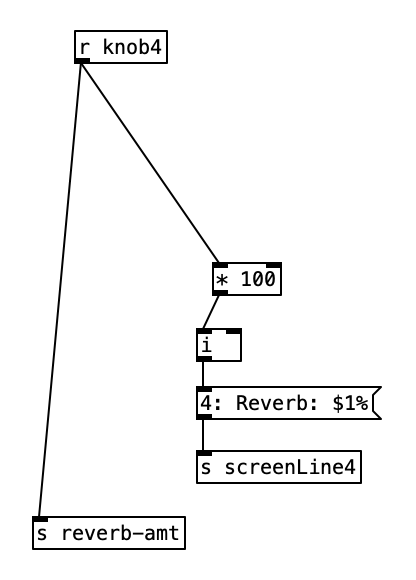
The phase vocoder part of the algorithm is sufficiently difficult such that I won’t attempt to go through it here, rather I will go through the reverb portion of the patch. As stated previously, knob four controls the balance between the dry (non-reverberated) and the reverberated sound. Thus value is then sent to the screen as a percentage, and is also sent to the variable reverb-amt using a number from 0 to 1 inclusive.

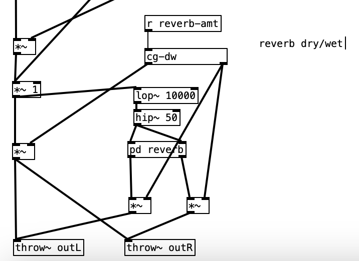
When the value of reverb-amt is recieved, it is sent to a subroutine called cg-dw. I’m not sure why the author of the patch used that name (perhaps cg stands for constant gardener), but this subroutine basically splits the signal in two, and modifies the value the will be returned out of the left outlet to be the inverse of the value of the right outlet (that is 1 – the reverb amount). Both values are passed through a low pass filter with cutoff frequency of 5 Hz, presumably to smooth out the signal.

The object lop~ 10000 receives its input from a chain that can be traced back to the input of the dry audio coming from the Organelle’s audio input. This object is a low pass filter, which means that the frequencies below the cutoff frequency, in this case 10,000 Hz, to pass through the filter, which in return attenuates the frequencies above the cutoff frequency. More specifically, lop is a one-pole, which means that the amount of attenuation is 6 dB per octave. A reduction of 6 dB effectively is half the power of the original. Thus, if the cutoff frequency of a low pass filter is set to 100 Hz, the power at 200 Hz (doubling a frequency raises the pitch an octave) is half of what it would normally be, and at 400 Hz, the power would be a quarter of what it would normally be.

In analog synthesis a two pole (12 dB / octave reduction) or a four pole (24 dB / octave) filter would be considered more desirable. Thus, a one pole filter can be thought of as a fairly gentle filter. This low pass filter is put in the signal chain to reduce the high frequency content to avoid aliasing. Aliasing is the creation of artifacts when a signal is not sampled frequently enough to faithfully represent a signal. Human beings can hear up to 20,000 Hz, but audio demands at least one positive value and one negative value to represent a sound wave. Thus, CD quality sound uses 44,100 samples per second. The Nyquist frequency, the frequency at which aliasing starts is half the sample rate. In the case of CD quality audio, that would be 22,050 Hz. Thus, our low pass filter reduces these frequencies by more than half.

The signal is then passed to the object hip~ 50. This object is a one-pole high pass filter. This type of filter attenuates the frequencies below the cutoff frequency (in this case 50 Hz). Human hearing goes down to about 20 Hz. Thus, the energy at this frequency would be attenuated by more than half. This filter is inserted into the chain to reduce thumps and low frequency noise.

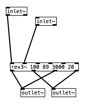
Finally we get to the reverb subroutine itself. The object that does most of the heavy lifting in this subroutine is rev~ 100 89 3000 20. This is a stereo input, four output reverb unit. Accordingly the first two inlets would be the left and right input. The other four inlets are covered by creation arguments (100 89 3000 20). These four values correspond to: output value, liveness, crossover frequency, and high frequency dampening. The output value is expressed in decibels. When expressed in this manner we can think of a change of 10 dB as doubling or halving the volume of a sound. We often consider the threshold of pain (audio so loud that it is physically painful to us) as starting around 120 dB. Thus, 100 dB, while considered to be loud, is 1/4 as loud as the threshold of pain. The liveness setting is really a feedback level (how much of the reverberated sound is fed back through the algorithm). A setting of 100 would yield reverb that would go on forever, while the setting 80 would give us short reverb. Accordingly, 89 gives us a moderate amount of reverb.

The last two values, cross over frequency and high frequency dampening work somewhat like a low pass filter. In the acoustic world low frequencies reverberate very effectively, while high frequencies tend to be absorbed by the environment. That is why a highly reverberant space like a cave or a cathedral has a dark sound to its reverb. In order to model this phenomenon, most reverb algorithms have an ability to attenuate high frequencies built into them. In this case 3,000 Hz is the frequency at which dampening begins. Here dampening is expressed as a percentage. Thus, a dampening of 0 would mean no dampening occurs, while 100 would mean that all of the frequencies about the crossover frequency are dampened. Accordingly, 20 seems like a moderate value. The outlets from pd reverb are then multiplied by the right outlet of cg-dw, applying the amount of reverb desired, and sent to the right and left outputs using throw~ outL and throw~ outR respectively.

For the EYESY I used the patch Mirror Grid Inverse – Trails. The EYESY’s five knobs are used to control: line width, line spacing, trails fade, foreground color, and background color. EYESY programming is accomplished in the language Python, and utilizes subroutines included in a library designed for creating video games called pygame.

An EYESY program is typically in four parts. The first part is where Python libraries are imported (pygame must be imported in any EYESY program). This particular program imports: os, pygame, math, and time. The second part is a setup function. This program uses the code def setup(screen, etc): pass to accomplish this. The third part is a draw function, which will be executed once for every frame of video. Accordingly, while this is where most of the magic happens, it should be written to be as lean as possible in order to run smoothly. Finally, the output should be routed to the screen.

In terms of the performance, I occasionally used knob 2 to change the pitch. I left reverb at 100%, and mix around 50% for the duration of the improvisation. I could have used the keyboard of the Organelle to play specific pitched versions of the audio input. Next month I hope to tackle additive synthesis, and perhaps use a webcam with the EYESY. Given that I’ve given a basic explanation of the first two parts of an EYESY program, in future months I hope to go through EYESY programs in greater detail.

Experiment 2: Analog Style


May has been a busy month for me. Thus, my second experiment in my project funded by Digital Innovation Lab at Stonehill College investigates the use of the preset patch Analog Style (designed by Critter and Guitari). To be specific, I am using a WARBL wind controller with EVI fingering to control the patch. I am using the breath control on the WARBL to control the cutoff frequency of Analog Style (using MIDI controller 24).

Due to the busyness of the end of the semester, this experiment features no original programming on the organelle. However, I did create a program in Pure Data to create accompaniment and drive the EYESY. To accompany the experiment, I used the H.E.A.P, the Housatonic Electronic Algorithmic Philharmonic. This a fun, frivolous name I’ve given to a small, battery powered synthesizer / sampler setup I’ve assembled for live performance. It consists of three synthesizers / samplers: a Volca Sample 2 (which provides 10 channels of late 1980s style lo fidelity digital sampling), a Volca Keys (which can be used as an analog monophonic or 3 note polyphonic synthesizer), and a Volca FM 2 (which is a clone of the 1980s classic, the Yamaha DX7, the best selling synthesizer of all time). I’ve also begun to think of the EYESY, as we’ll see later, as part of the H.E.A.P.

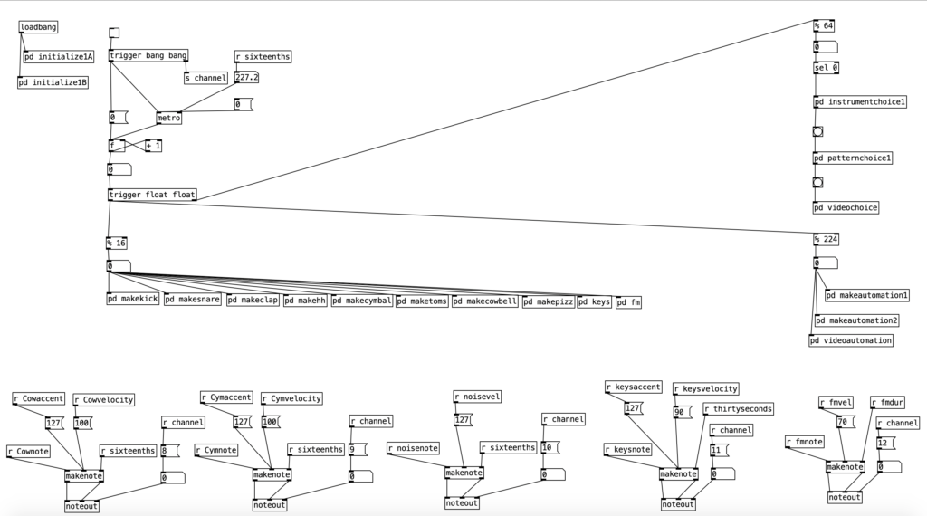
I won’t go into great detail about the program that generates the accompaniment for Experiment 2, as I have other blog posts that go into detail about various algorithms included in the program. Ultimately, the program is intended to generate relatively generic, but fairly usable R&B esque slow jams. The music is in common time using sixteenth notes. The portion of the program including and beneath % 16 (mod 16) ensures that the resulting music will have 16 pulses per measure. Likewise, the instrumentation and musical patterns change every four measures. This is enabled by the part of the program including and beneath % 64 (four measures of sixteenth notes adds up to 64).

The Volca Sample is being used to provide the drum beat, and some string pizzicato (see pd makepizz). The Volca Keys provides some synthesized bass patterns that run two measure loops. The Volca FM provides four chord, four note chord progressions that repeat every two measures. To create these chord progressions I used some music programming techniques that I’ve covered in a previous blog entry, though in this experiment I am use the brass friendly key of G minor.

One of the newer programming tricks I used in this program is an algorithm designed to drive the EYESY. While the EYESY generates hypnotic, interactive video animations, left to its own devices it can get a bit repetitive fairly quickly. In order to generate anything that seems even remotely dynamic some one needs to perform the EYESY by rotating its five knobs. This is an impossibility for any performing musician, save for a vocalist. Thankfully, we can do the equivalent of turning the knobs on the EYESY through MIDI using controllers 21 through 25.

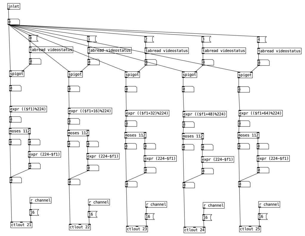
The algorithm I’ve created to drive the EYESY is designed to make slow, evolving changes. To control these changes I’ve created a table called videostatus. It consists of five positions that contain a one or a zero to denote whether changes should be make or not made to a given knob during the current four measure phrase.

The subroutine pd videochoice is triggered at the beginning of every four measure phrase. It generates five different random numbers that are either a zero or a one. These results are then stored in the table videostatus.

The subroutine pd videoautomation updates the knob positions on the EYESY once every sixteenth note. It is passed the current sixteenth note number modded by the number 224, which corresponds to 14 measures of sixteenth notes. The subroutine contains five nearly identical columns, each of which corresponds to each of the five knobs on the EYESY. First the algorithm checks the current states of each of the five positions of videostatus table. When that value is one, that allows the current sixteenth note number to pass through the spigot. This value is passed through an expr statement that displaces the sixteenth note number. The column corresponding to knob one is not displaced, but each subsequent column is displaced by one measure (16 sixteenths), which is then modded to stay between 0 and 224. The statement moses 112 is used to determine whether we should be counting up to 112, or counting down to 0. This is accomplished by having numbers that are greater than 112 to pass through expr (224-$f1), which causes the result to get small as the input value is increased. The result of this is then passed to one of the five controller values (21-25) on MIDI channel 16 (the channel I’ve set my EYESY to).

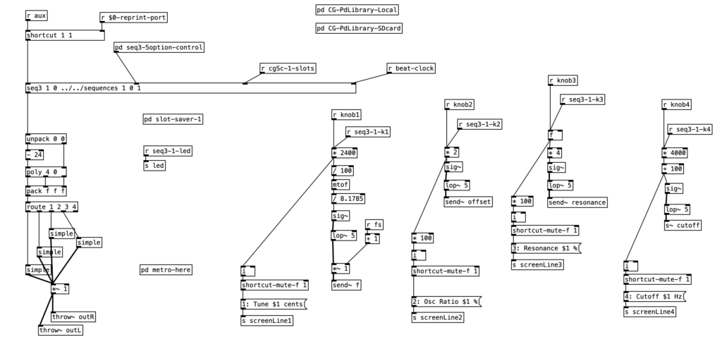
Since I went over the mother patch in the previous experiment, I’ll start with going over main.pd for the Analog Style patch. We can see that knob one controls the tuning of the patch, while knob two creates an offset frequency for a second oscillator. The third knob sets the resonance of the low pass filter, while the fourth knob (the one I am controlling using the WARBL) sets the cutoff frequency of filter. To learn more about what low pass filters are, check out my blog entry on Low Pass Filters in LogicPro. However, to summarize briefly in relationship to the WARBL, when the amount of breath coming through is low, that in turn sets the cutoff frequency to be low as well, resulting in less sound (and only low frequency sound) to come out of the Organelle.

We can also see that this patch allows for sequencing when the aux button is down. However we will not go through how sequencing works today. We will however go into simple, which is the subroutine that creates the sound. We can see two oscillators, blsaw, in this subroutine that generate sawtooth waves. For more information on subtractive synthesis waveforms (including sawtooth waves), check out my blog entry on Subtractive Synthesis Waveforms in Logic Pro. One of those two blsaw oscillators is modified by the offset of knob two. The mixture of these two oscillators is passed to a low pass filter, moog~. This object also receives a center frequency to its center inlet, and a resonance value to its right most inlet. The outlet of this object is then attenuated slightly, *~ .75, before being sent to the subroutine’s outlet.

Again, I’ve found that the accompaniment generated by experiment.pd to be generic, but also fairly usable. It should be relatively easy to change the tempo, phrase length, or any number of musical patterns to create music that is stylistically different. Also, I enjoy slow evolving nature of EYESY generated video. I feel that turning on and off changes to various combinations of the five knobs add a degree of subtlety that aid in the dynamic nature of the video.

I am disappointed in my performance on the WARBL. I am still getting used to the EVI fingering on the instrument, so there are some very sour notes from time to time. However, I am very pleased with the range of the WARBL, as well as the subtle breath control the instrument provides. The fingering makes jumping octaves and fifths very easy. In future experiments I hope to get into hacking existing Organelle patches. I also plan to come up with variants of the videoautomation algorithm to create more sudden, less subtle changes to the EYESY’s settings.